Denoisers and Plug-and-Play

Plug-and-Play (PnP) methods reconstruct with an iterative algorithm in which a denoiser takes the place of a regulariser. The denoiser is trained once, on clean images with added Gaussian noise, and works for any operator: the operator only appears in the algorithm.

This tutorial trains a denoiser with GaussianDenoiserSolver and reconstructs with it (LION.reconstructors.PnP). Short runs, to show how.

Previous: Self-supervised training. Next: Learned regularisers.

Needs a GPU and the processed LIDC-IDRI data in LION_DATA_PATH; downloads the authors’ trained DRUNet (130 MB).

Note

The models trained in these tutorials are toys: a few epochs on a few slices, to show how LION is used, so their results are poor (often worse than FDK). Trained as their papers train them (many epochs, all the data), they do what the papers report.

The data and the denoiser

The denoiser only uses the clean images (the targets of the experiment’s samples). DRUNet (Zhang et al., 2021) takes the noise level as an input, so one network denoises every level.

import tempfile

import matplotlib.pyplot as plt
import torch
from torch.utils.data import DataLoader, Subset

from LION.experiments import ct_experiments
from LION.metrics.psnr import PSNR
from LION.models.CNNs.drunet import DRUNet
from LION.optimizers.GaussianDenoiserSolver import GaussianDenoiserSolver

experiment = ct_experiments.LowDoseCTRecon()
training = Subset(experiment.get_dataset("train"), range(40))
validation = Subset(experiment.get_dataset("validation"), range(8))

training_loader = DataLoader(training, batch_size=4, shuffle=True)
validation_loader = DataLoader(validation, batch_size=4)

parameters = DRUNet.default_parameters()
parameters.use_noise_level = True
denoiser = DRUNet(parameters)

/mhome/damtp/r/ab2860/AItomotools/LION/data_loaders/LIDC_IDRI.py:487: UserWarning: LIDC-IDRI: left out 2 damaged or unusable files (re-run the pre-processing for these patients): ['LIDC-IDRI-0238 (not resampled)', 'LIDC-IDRI-0585 (not resampled)']
  warnings.warn(

Noise levels are in the units the denoiser sees. The literature’s (k/255) are for images in [0, 1], so the images are normalised to [0, 1] by their range over the training data. The normalisation is saved with the model and applied whenever it is used.

denoiser.set_normalisation("dataset", training)

Training the denoiser

GaussianDenoiserSolver adds the noise. Its parameters follow the literature: one noise level per image, drawn from a range; random flips and rotations; optionally random crops (patches) and random erasing; fixed noise levels to validate at.

solver_parameters = GaussianDenoiserSolver.default_parameters()
solver_parameters.noise_level = [0.0, 50 / 255]
solver_parameters.patches = GaussianDenoiserSolver.patches(8, 128)  # 8 crops a slice
solver_parameters.validation_noise_levels = [15 / 255, 25 / 255]
print(solver_parameters)

noise_level : [0.0, 0.19607843137254902]
patches : n_patches : 8
patch_size : 128
augment : True
random_erasing : False
validation_noise_levels : [0.058823529411764705, 0.09803921568627451]

It doesn’t use the operator, but takes its parameters, recorded as the problem the denoiser was trained for.

folder = tempfile.mkdtemp()
solver = GaussianDenoiserSolver(
    denoiser,
    torch.optim.Adam(denoiser.parameters(), lr=1e-4),
    torch.nn.L1Loss(),
    operator_params=experiment.operator_params,
    solver_params=solver_parameters,
)
solver.set_training(training_loader)
solver.set_validation(validation_loader, 1, PSNR(), validation_fname="DRUNet_best")
solver.set_saving(folder, "DRUNet")
solver.train(3)
solver.save_final_results()

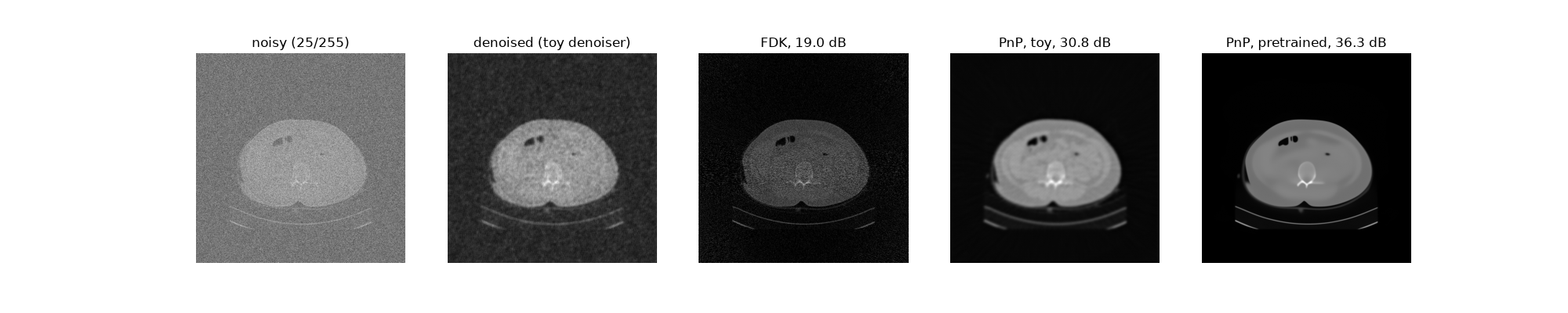
Denoising a validation image at 25/255. LION’s solvers and reconstructors normalise for the model; called by hand, the model takes normalised images:

image = validation[0][1]
x = denoiser.normalise(image[None])  # to [0, 1], as the denoiser sees it
noisy = x + 25 / 255 * torch.randn_like(x)
denoiser.eval()
with torch.no_grad():
    denoised = denoiser(noisy, noise_level=25 / 255)

Jacobian penalties

PnP methods are proven to converge when the denoiser has a property a network doesn’t have on its own: being firmly nonexpansive (Pesquet et al., 2021) or a proximal operator (Hurault et al., 2022). A penalty on the denoiser’s Jacobian, given to the solver as its model_regularization, trains it towards that. Both papers add it after training without it, e.g. fine-tuning the trained denoiser:

from LION.losses.jacobian_penalty import FirmlyNonexpansivePenalty

solver = GaussianDenoiserSolver(
    denoiser,
    torch.optim.Adam(denoiser.parameters(), lr=1e-5),
    torch.nn.L1Loss(),
    operator_params=experiment.operator_params,
    solver_params=solver_parameters,
    model_regularization=FirmlyNonexpansivePenalty(),  # off by default
)

The gradient-step denoiser (LION.models.PnP.gradient_step_denoiser.GSD) wraps any denoiser N as x - grad g(x), g(x) = ½||x - N(x)||², for Hurault et al.’s ProximalDenoiserPenalty.

Plug-and-Play reconstruction

PnP takes the operator (or its parameters), the denoiser and the algorithm’s parameters: ADMM, HQS or FBS (forward-backward splitting).

from LION.operators.ct import fdk
from LION.reconstructors.PnP import PnP

pnp_parameters = PnP.default_parameters("ADMM")
print(pnp_parameters)
pnp_parameters.max_iter = 20
pnp_parameters.noise_level = 10 / 255  # the denoiser's, in its [0, 1] units
# eta, ADMM's weight between the data and the prior, is by default relative to
# the operator: 1e-2 ||A||² (larger trusts the prior more)
pnp = PnP(experiment.operator_params, denoiser, pnp_parameters)

sinogram, image = validation[0]
reconstruction = pnp.reconstruct(sinogram)
# or one algorithm with its settings given:
# reconstruction = pnp.admm_algorithm(sinogram, max_iter=20, noise_level=10 / 255)

algorithm : ADMM
initial_reconstruction : default
eta : None
max_iter : 10
cg_max_iter : 100
cg_tol : 1e-07
noise_level : None

A pretrained denoiser

The denoiser above is a toy, trained for 3 epochs on 40 slices: a poor prior. The DRUNet its authors trained on natural images (a 130 MB download, on images in [0, 1]) is a good one, and the same reconstructor with it shows what PnP does:

pretrained = DRUNet.pretrained()
pretrained.set_normalisation("dataset", training)
pnp_pretrained = PnP(experiment.operator_params, pretrained, pnp_parameters)
pretrained_reconstruction = pnp_pretrained.reconstruct(sinogram)

HQS and FBS are used the same way:

hqs = PnP(experiment.operator_params, denoiser, PnP.default_parameters("HQS"))
print(PnP.default_parameters("FBS"))

algorithm : FBS
initial_reconstruction : default
step_size : None
max_iter : 10
noise_level : None

psnr = PSNR()
fbp = fdk(sinogram, experiment.operator_params)
fig, axes = plt.subplots(1, 5, figsize=(20, 4))
shown = [
    ("noisy (25/255)", noisy[0]),
    ("denoised (toy denoiser)", denoised[0]),
    (f"FDK, {psnr(fbp, image, batched=False):.1f} dB", fbp),
    (f"PnP, toy, {psnr(reconstruction, image, batched=False):.1f} dB", reconstruction),
    (
        f"PnP, pretrained, {psnr(pretrained_reconstruction, image, batched=False):.1f} dB",
        pretrained_reconstruction,
    ),
]
for ax, (title, x) in zip(axes, shown):
    ax.imshow(x[0].cpu(), cmap="gray")
    ax.set_title(title)
    ax.axis("off")

A reconstructor is saved with pnp.save(file): its settings, and its model by the file it was loaded from (Saving, loading and records).