Operators: CT geometry, projections and reconstructions

Everything in LION starts from a forward operator: the map from what we want (the image) to what we measure (for CT, the sinogram). This tutorial builds a CT geometry, makes its operator, simulates noisy measurements and reconstructs them with classical methods.

The words LION uses are general, as an operator can be anything: its domain is what it is applied to (here the image), its range what it gives (here the sinogram). Next: Parameters and specs.

Needs a GPU: LION’s CT operator projects with tomosipo and ASTRA.

A phantom

Any image works; here the Shepp-Logan phantom, with values like densities in g/cm³ (water is 1), the units LION’s CT data are in.

import matplotlib.pyplot as plt
import torch
from skimage.data import shepp_logan_phantom
from skimage.transform import resize

from LION.utils.device import default_device

# LION puts its tensors on default_device(): the GPU if there is one (set
# another with torch.cuda.set_device), the CPU otherwise.
device = default_device()

phantom = resize(shepp_logan_phantom(), (512, 512), anti_aliasing=True)
image = torch.tensor(phantom, dtype=torch.float32, device=device)[None]  # (1, H, W)
print(image.shape)

torch.Size([1, 512, 512])

The geometry

A Geometry holds everything about the scanner: source and detector distances (dso, dsd, in mm), the detector, the image and the angles. Geometry.default_parameters() is LION’s default: a fan beam with a 900-pixel detector, 512x512 images of 300 mm and 360 angles. Printing it shows every value.

from LION.operators.ct import Geometry

geometry = Geometry.default_parameters()
print(geometry)

CT Geometry
CT type/mode = fan
-----
Distance from source to detector (DSD) = 1050 mm
Distance from source to origin (DSO)= 575 mm
-----
Detector
Detector shape = [  1 900]
Detector size = [  1 900] mm
-----
Image
Image shape = [  1 512 512]
Image size = [  0.5859375 300.        300.       ] mm
Number of angles = (360,)

The image and the detector are each given by two of three values: the shape (pixels), the size (mm) and the spacing (mm per pixel). The third is computed, so it is never out of date: halving the image’s pixels doubles their size.

print(geometry.image_shape, geometry.image_size, geometry.voxel_size)
geometry.image_shape = [1, 256, 256]
print(geometry.image_shape, geometry.image_size, geometry.voxel_size)
geometry = Geometry.default_parameters()  # back to the default

[  1 512 512] [  0.5859375 300.        300.       ] [0.5859375 0.5859375 0.5859375]
[  1 256 256] [  0.5859375 300.        300.       ] [0.5859375 1.171875  1.171875 ]

Other presets: sparse view (50 angles), limited angle (60 angles over 60 degrees), and their parallel-beam versions.

sparse = Geometry.sparse_view_parameters()
limited = Geometry.sparse_angle_parameters()
parallel = Geometry.parallel_default_parameters()
print(len(sparse.angles), len(limited.angles), parallel.mode)

50 60 parallel

The operator

A geometry is the operator’s parameters: it makes the operator. The operator is a function of torch tensors: op(x) projects, op.adjoint(y) backprojects. Its domain_shape and range_shape say what they take.

op = geometry.make_operator()
print("domain:", op.domain_shape, "range:", op.range_shape)

sinogram = op(image)
backprojection = op.adjoint(sinogram)

fig, axes = plt.subplots(1, 3, figsize=(12, 4))
for ax, (title, x) in zip(
    axes,
    [("image", image), ("sinogram", sinogram), ("backprojection", backprojection)],
):
    ax.imshow(x[0].cpu(), cmap="gray", aspect="auto")
    ax.set_title(title)
    ax.axis("off")

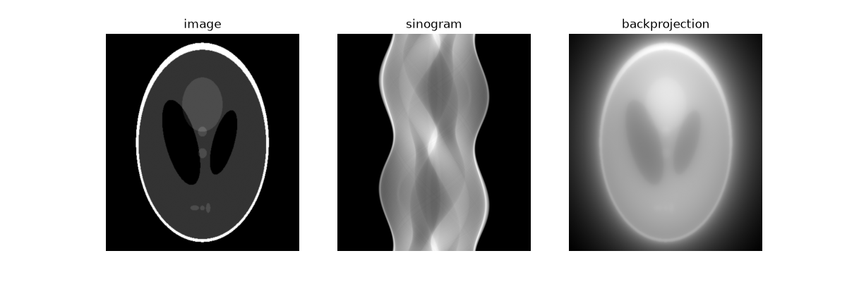
domain: (1, 512, 512) range: (1, 360, 900)

The operator itself takes one sample, (1, H, W). Batches, (B, 1, H, W), go through its autograd versions (below) and through LION’s reconstructions, models and solvers, which all take them.

Noise

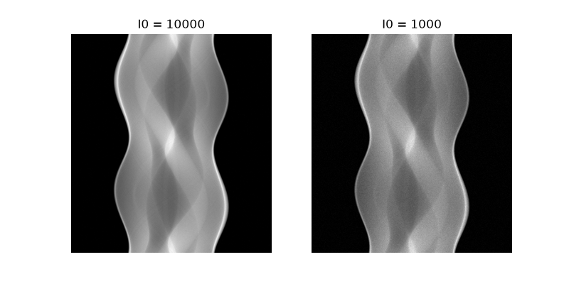
sinogram_add_noise simulates a scan: I0 photons per detector pixel (fewer: noisier), Poisson noise, the electronic noise and cross-talk of an energy-integrating detector. It needs the sinogram of densities in mm, as here. LION’s experiments use this with set doses (Data and experiments).

from LION.operators.ct.ct_utils import sinogram_add_noise

noisy = {I0: sinogram_add_noise(sinogram, I0=I0) for I0 in (10000, 1000)}

fig, axes = plt.subplots(1, 2, figsize=(8, 4))
for ax, (I0, y) in zip(axes, noisy.items()):
    ax.imshow(y[0].cpu(), cmap="gray", aspect="auto")
    ax.set_title(f"I0 = {I0}")
    ax.axis("off")

Reconstructions

LION’s CT reconstructions take the measurements and the operator (or its geometry): FDK (filtered backprojection), SIRT and TV minimisation, all from tomosipo’s algorithms, all batched.

from LION.operators.ct import fdk, sirt, tv_min

y = noisy[1000]
reconstructions = {
    "FDK": fdk(y, op),
    "SIRT, 100 iterations": sirt(y, op, num_iterations=100),
    "TV": tv_min(y, op, lam=1e-4, num_iterations=100, verbose=0),
}

fig, axes = plt.subplots(1, 3, figsize=(12, 4))
for ax, (title, x) in zip(axes, reconstructions.items()):
    ax.imshow(x[0].cpu(), cmap="gray", vmin=0, vmax=1)
    ax.set_title(title)
    ax.axis("off")

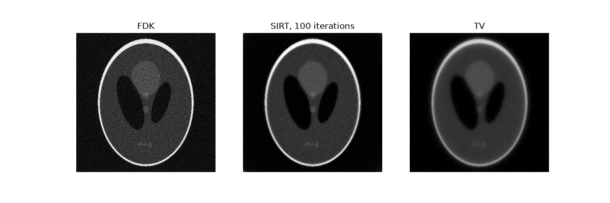
Each operator knows its usual reconstruction, default_reconstruction: FDK for CT. LION’s models, solvers and evaluations start from it unless told otherwise, so they work with any operator.

print(op.default_reconstruction_fn())
x0 = op.default_reconstruction(y)

<function fdk at 0x7f2b3c260220>

Training through the operator

Unrolled models (LPD, LG, …) differentiate through the operator. op.autograd() gives the projection and backprojection as torch autograd functions:

A, AT = op.autograd()  # on batches, (B, 1, H, W)
x = torch.zeros_like(image[None], requires_grad=True)  # a batch of one
loss = ((A(x) - y[None]) ** 2).mean()
loss.backward()
print(x.grad.shape)  # the gradient of the data fit, an image

batch = torch.stack([image, 2 * image])  # (2, 1, 512, 512)
print(A(batch).shape)

torch.Size([1, 1, 512, 512])
torch.Size([2, 1, 360, 900])

Many methods need the operator’s norm (its largest singular value), e.g. for step sizes; the power method estimates it.

from LION.utils.math import power_method

print(f"||A|| = {power_method(op):.1f}")

||A|| = 285.6

Splitting the measurements

Self-supervised methods (Noise2Inverse and others) split the sinogram by angles. The geometry splits itself, and the measurements to match:

angles = list(range(0, len(geometry.angles), 4))  # every 4th angle
quarter = geometry.split(angles)
y_quarter = geometry.split_measurements(y, angles)
print(len(quarter.angles), y_quarter.shape)
x_quarter = fdk(y_quarter, quarter)

90 torch.Size([1, 90, 900])

Other operators

CT is one operator. LION has others (LION.operators): wavelets, photocurrent mapping (LION.operators.pcm), composite and debiasing operators; any of them works with the classical algorithms, e.g. FISTA for sparse recovery. An operator is a class with forward, adjoint and its shapes: Extending LION writes one.

from LION.operators.Wavelet2D import Wavelet2D

wavelet = Wavelet2D((512, 512), wavelet_name="db4", device=device)
coefficients = wavelet(image[0])
print(
    coefficients.shape,
    torch.allclose(wavelet.inverse(coefficients), image[0], atol=1e-4),
)

torch.Size([262144]) True